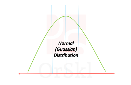
Normal distribution also known as Gaussian distribution is one of the core probabilistic models to data scientists. Naturally occurring high volume data is approximated to follow normal distribution. According to Central limit theorem, large volume of data with multiple independent variables also assumed to follow normal distribution irrespective of their individual distributions. In reality we deal with multi dimension data, we have most of the machine learning algorithms in the market are developed on the assumption that data is normally distributed.

This is one of the very important checks in process of building machine learning models (most commonly used models) to the data, if data is not normal then transformations might be required to the data to follow normal distribution.

In this blog we are not going to go through the theory of normal distribution, but find ways to identify if the given data set is normally distributed or not, in Python. Let us pick two randomly generated data sets as below, one normally distributed and other uniformly distributed.

import scipy.stats as orsklss
import numpy as orsklnp
import matplotlib.pyplot as orsklplt
mu, sigma = 0.5, 0.1
normdata = orsklnp.random.normal(mu, sigma, 100000)
unidata=orsklnp.random.uniform(0,1,10000)

Method 1 –  Skewness & Kurtosis test

orsklss.skewtest(normdata)
SkewtestResult(statistic=-0.04526696516442479, pvalue=0.9638945184142869)
orsklss.skew(normdata, axis=0)
-0.007548210116297582

Null hypothesis of this skewtest (two-tail test) is that input data follows symmetric data distribution over mean value. If p value is greater than 2.5% and less than 97.5% of significance level, data is considered to be symmetric. Function skew gives value close to 0 if data is approximately symmetric. This is one of the primary characteristics of normally distributed data.

orsklss.skewtest(unidata)
SkewtestResult(statistic=-0.4442986293221471, pvalue=0.6568266920987647)orsklss.skew(unidata, axis=0)-0.010875228659639516

But, uniformly distributed data is also symmetric over the mean. Hence using skewness alone will not help to conclude if data is normally distributed, so we use kurtosis as another metric. Kurtosis shows how intense is the bell curve over the mean, this exists for normally distributed data and not for uniform data.

orsklss.kurtosis(normdata, fisher=True)
-0.007548210116297582
orsklss.kurtosis(unidata, fisher=True)
-1.2304818179223689

Data which has kurtosis value close to 0 has bell shaped distribution and in this case normally distributed wins over uniform data. To identify if data is normally distributed using this method its skewness and kurtosis using the above functions should be close to 0.

Method 2 – D’Agostino and Pearson’s test

orsklss.normaltest(normdata)
NormaltestResult(statistic=0.23007063346940448, pvalue=0.8913346643210859)
orsklss.normaltest(unidata)
NormaltestResult(statistic=11802.268274443317, pvalue=0.0)

Both skewness and kurtosis of the data is tested in this method, it’s a chi squared two sided test with null hypothesis as data follows normal distribution. With 5% of default significance level, p value less than 2.5% and greater than 97.5% should fail to accept null hypothesis. In the output of the sample data, p-value for normally distributed data is 89% and uniform data is 0%. So we fail to reject the null hypothesis for normdata and reject the null hypothesis for unidata.

To identify if data is normally distributed using D’Agostino and Pearson’s test p value should be >= 2.5% and <= 97.5%

Method 3 – Shapiro-Wilk test

orsklss.shapiro(normdata)
(0.9999831318855286, 0.9685483574867249)
orsklss.shapiro(unidata)
(0.9513749480247498, 0.0)

Shapiro-Wilk test tests the data for normality with null hypothesis as ‘data follows normal distribution’. With significance level 5%, any p-value greater than 5% should be good to consider that data is normally distributed. But higher the p-value means the data is very much close to normal distribution.

Limitation of this test is that p-value might be misleading for data points greater than 5000, but in our example it was accurate as data perfectly follows normal distribution though there were 100000 data points. But for the real world data, this test would not be reliable for larger data set.

Method 4 – Anderson-Darling test

Anderson-Darling test is used to test multiple data distributions like Normal, Exponential, Logistic and few more. This statistical test will test with null hypothesis as ‘data is normally distributed’.

orsklss.anderson(normdata,dist=’norm’)
AndersonResult(statistic=0.176307244139025, critical_values=array([0.576, 0.656, 0.787, 0.918, 1.092]), significance_level=array([15. , 10. ,  5. ,  2.5,  1. ]))
orsklss.anderson(unidata,dist=’norm’)
AndersonResult(statistic=123.5706536716898, critical_values=array([0.576, 0.656, 0.787, 0.918, 1.092]), significance_level=array([15. , 10. ,  5. ,  2.5,  1. ]))

For significance level of 5%, its respective critical value for normally distributed data is 0.918 in the output. If the statistic value is far greater than its respective critical value, then you can reject the null hypothesis.

In our example, normdata statistic 0.176 is far less than its 5% critical value 0.918, hence we fail to reject null hypothesis. On other side unidata statistic 123.5 is far greater than its 5% critical value 0.918 and hence we reject null hypothesis that data follows normal distribution.

Conclusion:

• Am sure of few or more methods as well to identify if data follows normal distribution, but above four are most commonly used
• To make sure if test result is accurate, we tend to use multiple methods on the same data set to conclude if data is normally distributed
• Of the above methods, Shapiro-Wilk test can handle multi-dimensional data to test normality and others are uni-dimensional

Do you wish to watch video for the same? Here you go.